The RIAA curve

I am guessing most of my readers know what the RIAA EQ curve is—a 20dB boost to the high frequencies and a 20dB cut to the low frequencies when mastering a vinyl record, and then the opposite when playing it back.

Together, the cut and boost add up to a 40dB difference in equalization. That's quite the range and one of the first lessons we learned at the beginning of PS Audio's 50 year journey was the importance of that accuracy.

For the first year of our company's existence we spent it not selling products—because we didn't actually have anything ready for sale—but designing and figuring out how to build a phono stage that, despite its low cost, could whoop the sonic pants off the competition.

Not an easy task.

What we learned about RIAA accuracy came at the hands of one of our early mentors, Dr. Larry Stewart—a brilliant electrical engineer dedicated to designing sound generating equipment that would scare birds away from airports and vineyards.

Before Dr. Stewart, Stan and I would attempt to calculate the filter values of this curve using a conventional easy to understand formula that looks like this:

• fc​: Cutoff frequency in Hertz (Hz).
• $R$: Resistance in ohms (Ω).
• $C$: Capacitance in farads (F).

Pretty simple to find the reciprocal of 2π x the R and C in the circuit and work it backwards to figure out the appropriate values for the curve. Trouble was, there are multiple "poles" in the RIAA curve—3 to be exact. In simple terms, "poles" in a filter are specific frequencies where the filter changes how it amplifies or attenuates a signal. Think of a pole as a "turning point" in the filter's response.

Whatever we tried we could never get the curve just right and it was easy to hear even the small inaccuracies we wound up with.

Stan and I were at a loss (remember, this was before the internet and easy access to information—and we were hardly math wizards). Enter Dr. Stewart who had never heard of an RIAA curve but told us if we could supply the three turnover frequencies of the filter—50Hz (3,180 µs), 500Hz (318 µs), and 2,120Hz (75 µs)—he'd crank out a perfect one for us.

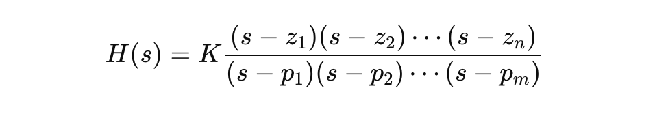
The filter he generated used a more sophisticated mathematical approach using Poles and Zeroes. 

• Poles: These are the values in the complex plane where the filter’s transfer function goes to infinity. Poles influence the stability and the frequency response of the filter.
• Zeroes: These are the values in the complex plane where the filter’s transfer function goes to zero. Zeroes control the notches in the frequency response.

The transfer function $H(s)$ or $H(z)$ of the filter is given by the ratio of the product of terms corresponding to zero locations to the product of terms corresponding to pole locations.

$$H(s) = K \frac{(s - z_1)(s - z_2)\cdots(s - z_n)}{(s - p_1)(s - p_2)\cdots(s - p_m)}$$

(s−p1​)(s−p2​)⋯(s−pm​)(s−z1​)(s−z2​)⋯(s−zn​)​

Where:

• $s$ is the complex frequency variable for analog filters.
• $z_i$ are the zeroes of the filter.
• $p_i$ are the poles of the filter.
• $K$ is a gain constant.

Ok, lots of gobbledygook. Basically, using this method you can calculate about anything involving multiple EQs and get accuracy down to a gnat's ass.

Bottom line? Using two precision resistors and capacitors we could build a passive RIAA curve with an accuracy of 0.01% (compared to about 1.5% before).

Sonically? It made all the difference in the world.

I still hate math.